增加复杂性
We can improve the resolution of the measurements by replacing the ruler with a micrometer having a fine-thread screw, so that we can resolve one-thousandths or even one ten-thousandths of an inch. Now, as we re-run the experiment, we can easily see, by simple visual inspection of the data, that it will not exactly fit on a straight line.
| Weight | Mark |
| 0 | 0.500 |
| 1 | 1.509 |
| 2 | 2.516 |
| 3 | 3.511 |
| 4 | 4.495 |
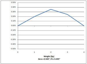
When we look closely at the deviation of the data from our hoped-for straight line, we can see that the differences are so small that they are less than the thickness of the graph line. Such a graph would not be useful, since it would not portray any useful information except a gross representation of the zero intercept and slope of the spring’s characteristics. Therefore, in order to present the data in a meaningful form, it is necessary to modify our classical idea about the graphing of data. We will need to magnify the scaling of the graph in such a way that the deviations from a straight line are easier to see.
Rather than graphing “Weight” versus “Deflection,” we can plot “Weight” versus “Deviation from a Straight Line.” Then, it becomes necessary to choose which straight line to use as a reference. One common choice is the “End Points Straight Line,” which is the line passing through the point at zero load and the point at maximum load.
As you can see in Figure 3, the horizontal axis represents the straight line we have chosen to use as a reference. But, notice, we have given up the scaling information about the spring. We can’t calculate the “pounds per inch” constant of the spring from the graphed information. Therefore, for the graph to be most useful, we should print the scaling constant somewhere on the graph.
Also, if we choose “Deviation” for the vertical axis, it is not too useful, since we can’t relate the numbers to the performance of the spring without dividing all the numbers by the full scale output range of the test. We can help the user of the graph by performing that division ahead of time, converting the units on the vertical axis to “Percent of Full Scale.” In our example, we would divide all the deviation numbers by 4.495 (that is: 4.995 – 0.500), the range of the test outputs from no load to full load.
By using “Percent of Full Scale,” we can easily compare the performance of many springs in a way which lets us select the ones which have the characteristics we want. Later on, we will see that springs have many more parameters than just the simple spring constant which was presented earlier in the deflection equation for springs.

Figure 3. Deviation from straight line versus applied weight.
You will notice that our new graph in Figure 3 gives us a much clearer pi


